ファイル:Newton iteration.png

ページのコンテンツが他言語でサポートされていません。
出典: フリー教科書『ウィキブックス(Wikibooks)』

元のファイル(2,406 × 1,978 ピクセル、ファイルサイズ: 55キロバイト、MIME タイプ: image/png)

このファイルはウィキメディア・コモンズから来ており、他のプロジェクトで使用されている可能性があります。 ウィキメディア・コモンズでのファイル解説ページにある説明を以下に示します。

概要

このファイルのベクター画像 (SVG) が利用できます。 使う目的に対し、元画像よりもSVGがより優れている場合、SVG画像を使用して下さい。

File:Newton iteration.png → File:Newton iteration.svg
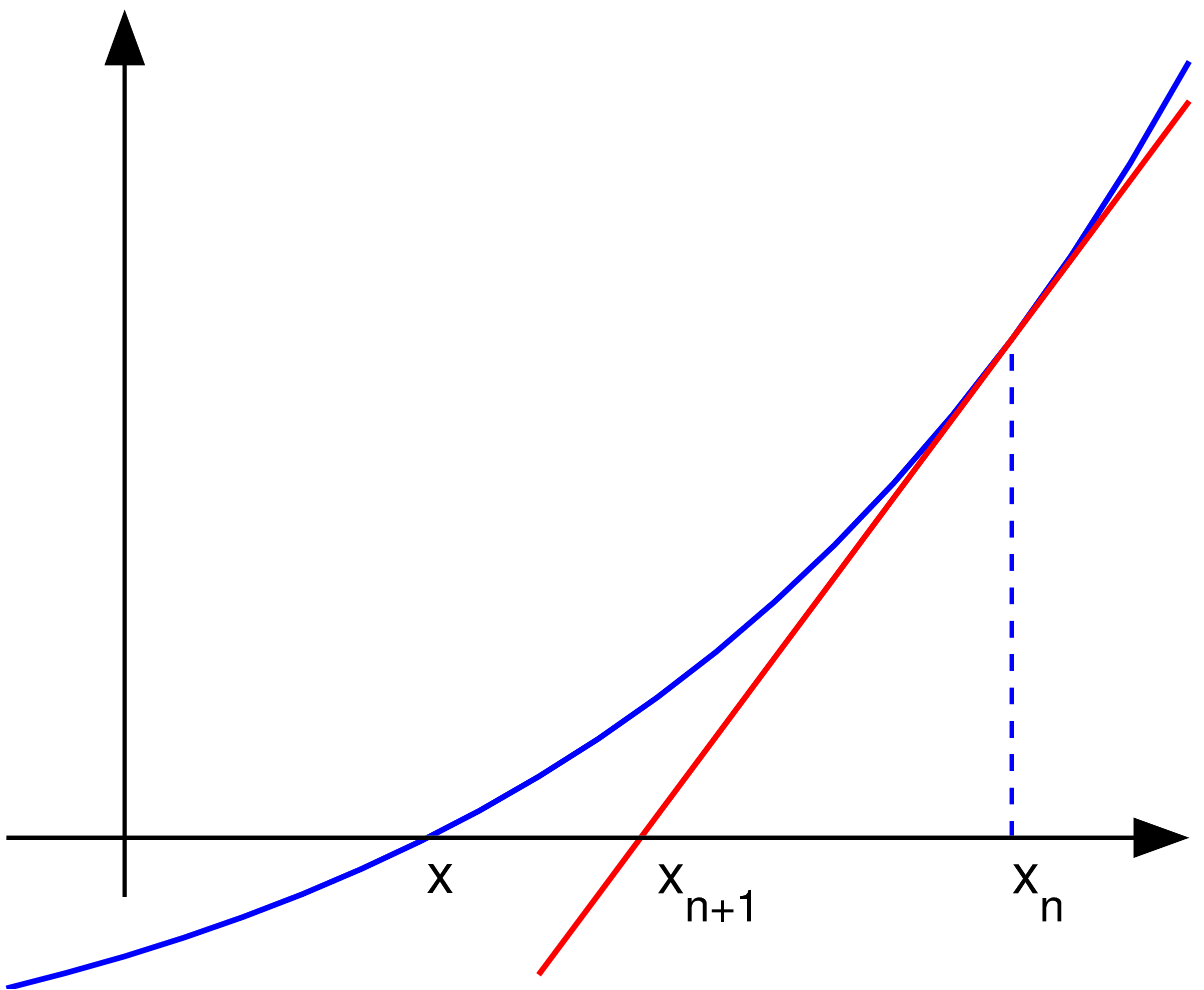
ベクターグラフィックスの詳細については、コモンズのSVG変換を参照ください。
SVGのMediaWikiのサポートに関する情報もあります。

他言語
Alemannisch  Bahasa Indonesia  Bahasa Melayu  British English  català  čeština  dansk  Deutsch  eesti  English  español  Esperanto  euskara  français  Frysk  galego  hrvatski  Ido  italiano  lietuvių  magyar  Nederlands  norsk bokmål  norsk nynorsk  occitan  Plattdüütsch  polski  português  português do Brasil  română  Scots  sicilianu  slovenčina  slovenščina  suomi  svenska  Tiếng Việt  Türkçe  vèneto  Ελληνικά  беларуская (тарашкевіца)  български  македонски  нохчийн  русский  српски / srpski  татарча/tatarça  українська  ქართული  հայերեն  বাংলা  தமிழ்  മലയാളം  ไทย  한국어  日本語  简体中文  繁體中文  עברית  العربية  فارسی  +/−
新しいSVG画像

解説 Uploader graphed this with en:MATLAB (Illustration of en:Newton's method)
日付 2004年11月22日 (first version); 2004-11-23 (last version)
原典 en.wikipedia からコモンズに移動されました。
作者 英語版ウィキペディアOlegalexandrovさん
PNG 開発
InfoField
 
この 図式MATLABで作成されました。
ソースコード
InfoField

MATLAB code

(Newton iteration)
% illustration of Newton's method for finding a zero of a function

function main ()
   
a=-1; b=1;   % interval endpoints
fs=20;       % text font size

% arrows settings
thickness1=2; thickness2=1.5; arrowsize=0.1; arrow_type=1;
angle=20; % in degrees

h=0.1;  % grid size
X=a:h:b; % points on the x axis
f=inline('exp(x)/1.5-0.5');   % function to plot
g=inline('exp(x)/1.5');       % derivative of f
x0=0.7; y0=f(x0);             % point at which to draw the tangent line 
m=g(x0);
Y=f(X);                       % points on the function to plot
XT=-0.1:h:b; YT=y0+(XT-x0)*m; % tangent line

% prepare the screen
clf; hold on; axis equal; axis off

% plot the graph and the tangent lines
plot(X, Y, 'linewidth', thickness1)
plot(XT, YT, 'r', 'linewidth', thickness1)
plot([x0 x0], [0, y0], '--', 'linewidth', thickness2)

% axes
small=0.2;
arrow([a 0], [b, 0], thickness2, arrowsize, angle, arrow_type, [0, 0, 0])
arrow([a+small, -0.1], [a+small, 1.4], thickness2, arrowsize, angle, arrow_type, [0, 0, 0])

% text
H=text(-0.29, -0.06,  'x'); set(H, 'fontsize', fs)
H=text(0.1, -0.1,  'x_{n+1}'); set(H, 'fontsize', fs)
H=text(0.7, -0.1,  'x_{n}'); set(H, 'fontsize', fs)

% save to disk
saveas(gcf, 'newton_iteration.eps', 'psc2')

function arrow(start, stop, thickness, arrow_size, sharpness, arrow_type, color)

% Function arguments:
% start, stop:  start and end coordinates of arrow, vectors of size 2
% thickness:    thickness of arrow stick
% arrow_size:   the size of the two sides of the angle in this picture ->
% sharpness:    angle between the arrow stick and arrow side, in degrees
% arrow_type:   1 for filled arrow, otherwise the arrow will be just two segments
% color:        arrow color, a vector of length three with values in [0, 1]

% convert to complex numbers
   i=sqrt(-1);
   start=start(1)+i*start(2); stop=stop(1)+i*stop(2);
   rotate_angle=exp(i*pi*sharpness/180);

% points making up the arrow tip (besides the "stop" point)
   point1 = stop - (arrow_size*rotate_angle)*(stop-start)/abs(stop-start);
   point2 = stop - (arrow_size/rotate_angle)*(stop-start)/abs(stop-start);

   if arrow_type==1 % filled arrow

      % plot the stick, but not till the end, looks bad
      t=0.5*arrow_size*cos(pi*sharpness/180)/abs(stop-start); stop1=t*start+(1-t)*stop;
      plot(real([start, stop1]), imag([start, stop1]), 'LineWidth', thickness, 'Color', color);

      % fill the arrow
      H=fill(real([stop, point1, point2]), imag([stop, point1, point2]), color);
      set(H, 'EdgeColor', 'none')

   else % two-segment arrow
      plot(real([start, stop]), imag([start, stop]),   'LineWidth', thickness, 'Color', color);
      plot(real([stop, point1]), imag([stop, point1]), 'LineWidth', thickness, 'Color', color);
      plot(real([stop, point2]), imag([stop, point2]), 'LineWidth', thickness, 'Color', color);
   end

ライセンス

Public domain この著作物は、著作者である英語版ウィキペディアOlegalexandrovさんによって権利が放棄され、パブリックドメインとされました。これは全世界で適用されます。
一部の国では、これが法的に可能ではない場合があります。その場合は、次のように宣言します。
Olegalexandrovは、あらゆる人に対して、法により必要とされている条件を除き、如何なる条件も課すことなく、あらゆる目的のためにこの著作物を使用する権利を与えます。


元のアップロードログ

元のファイルページはこちら。以下の利用者は全てen.wikipediaに属します。
  • 2004-11-23 19:55 Olegalexandrov 405×340×8 (14290 bytes) Scaled down the picture of Newton's method
  • 2004-11-22 21:34 Olegalexandrov 509×406×8 (16510 bytes) I graphed this with Matlab (Illustration of Newton's method) {{PD}}

キャプション

このファイルの内容を1行で記述してください

このファイルに描写されている項目

題材

ファイルの履歴

過去の版のファイルを表示するには、その版の日時をクリックしてください。

日付と時刻サムネイル寸法利用者コメント
現在の版2007年5月25日 (金) 03:232007年5月25日 (金) 03:23時点における版のサムネイル2,406 × 1,978 (55キロバイト)Oleg Alexandrov{{Information |Description=Uploader graphed this with en:MATLAB (Illustration of en:Newton's method) ==Source code== <pre> <nowiki> % illustration of Newton's method for finding a zero of a function function main () a=-1; b=1; % interva
2005年6月12日 (日) 23:112005年6月12日 (日) 23:11時点における版のサムネイル405 × 340 (6キロバイト)Everlongoptimized for smaller file size
2005年1月17日 (月) 23:062005年1月17日 (月) 23:06時点における版のサムネイル405 × 340 (14キロバイト)Andreas Ipp~commonswiki{{PD}}: Original author graphed this with MATLAB (Illustration of Newton's method), from Wikipedia.

このファイルを使用しているページはありません。

グローバルなファイル使用状況

以下に挙げる他のウィキがこの画像を使っています: